Regression using GPs

So far the examples have only considered the input space specified by the data . The GP class methods GeePea.GP.predict() and GeePea.GP.predictGP() return the predictive distributions of the GP:

y_pred, y_pred_err = gp.predict() # mean and kernel distribution
y_pred, y_pred_err = gp.predictGP() # assumes zero mean GP

There are also additional methods GeePea.GP.getRandomVector() and GeePea.GP.getRandomVectorFromPrior() to generate random draws from the posterior or prior:

yr = gp.getRandomVector() # get random vector from the posterior
yr = gp.getRandomVectorFromPrior() # get random vector from the prior

Note

These functions only return the predictive distributions for a single point estimate of the mean function parameters and kernel hyperparameters. Strictly speaking, this should take into account the posterior distribution of these parameters, but this is not easy to compute when using generic mean functions. This is generally fine for visualisation purposes, but a more rigorous treatment is necessary if using y_pred_err for further studies.

Note that these are called by GeePea.GP.plot() to obtain the model mean and predictive distribution.

We’ll start with a simple example:

x = [-1.50,-1.0,-0.75,-0.4,-0.25,0.00] #x data
y = [-1.6,-1.1,-0.5,0.25,0.5,0.8] #y data

hp = [0.,1.,0.3] #hyperparameters
fp = [0,0,1] #fix the noise parameter

#define the GP
gp = GeePea.GP(x,y,p=hp,fp=fp)

Then we can optimise and plot the GP:

gp.optimise()
gp.plot()

import GeePea
import numpy as np

#create test data
x = [-1.50,-1.0,-0.75,-0.4,-0.25,0.00]
y = [-1.6,-1.1,-0.5,0.25,0.5,0.8]

#define mean function parameters and hyperparameters
hp = [0.,1.,0.3] # kernel hyperparameters (sq exponential takes 3 parameters for 1D input)
fp = [0,0,1]

#define the GP
gp = GeePea.GP(x,y,p=hp,fp=fp)

#optimise and plot
gp.optimise()
gp.plot()

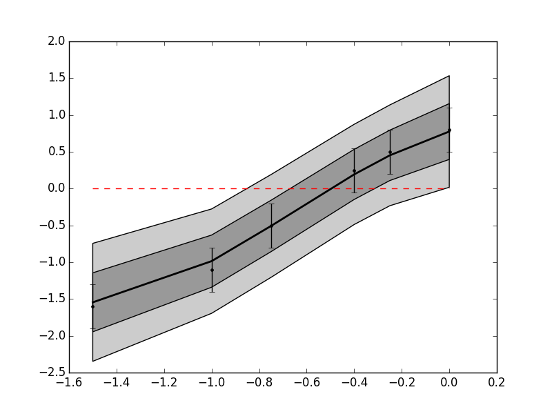
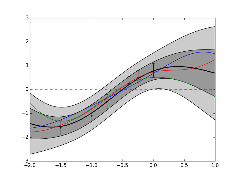
The predictive distribution is only returned for the 6 input data points, and therefore doesn’t look smooth as it should. We also might want to see how a model behaves further from the inputs. In order to do this, we can provide predictive inputs to the GP class:

x_p = np.linspace(-2,1,200) #predictive x inputs

gp = GeePea.GP(x,y,p=hp,fp=fp,x_pred=x_p)

or we can update a GP class (see note below):

gp.set_pars(x_pred=x_p)

Now when we make a prediction for our GP, the distribution will be plotted for x_p, and not x. We can also generate some random draws from the GP, e.g.:

for i in range(3): pylab.plot(gp.xmf_pred, gp.getRandomVector())

import GeePea
import numpy as np
import pylab

#create test data
x = [-1.50,-1.0,-0.75,-0.4,-0.25,0.00]
y = [-1.6,-1.1,-0.5,0.25,0.5,0.8]

#define mean function parameters and hyperparameters
hp = [0.,1.,0.3] # kernel hyperparameters (sq exponential takes 3 parameters for 1D input)
fp = [0,0,1]

#define the GP
gp = GeePea.GP(x,y,p=hp,fp=fp)

#also define a predictive distribution
x_p = np.linspace(-2,1,200)

#define the GP
gp.set_pars(x_pred = x_p)

#optimise and plot
gp.optimise()
gp.plot()

for i in range(3): pylab.plot(gp.xmf_pred, gp.getRandomVector())

Note

When using a mean function, the mean function arguments and predictive arguments can be set using xmf and xmf_pred if they are different to the kernel inputs (x and x_pred). By default, xmf and xmf_pred are set to x and x_pred respectively, and x_pred is set to x if it is also not defined. These can all be updated using GP.set_pars, but if redefining x_pred and xmf_pred, these should be done at the same time, otherwise they can be overwritten.