Inference of hyperparameters

In general, we don’t want a point estimate of the kernel hyperparamters and mean function parameters, but instead want to obtain the posterior distributions. This can easily be done using the GeePea.logLikelihood() and GeePea.logPosterior() methods, which can be used for optimisation and sampling the posterior using your favorite methods.

This simple example will follow on from the light curve example, and use MCMC functions from my ‘Infer’ module (also available from https://github.com/nealegibson/). See the Infer docstrings for more info, this will only give a simple MCMC eg. Just import the modules and define the light curve in the same way as before:

import numpy as np
import GeePea
import MyFuncs as MF
import Infer

time = np.linspace(-0.1,0.1,200)
mfp = [0.,2.5,11.,.1,0.6,0.2,0.3,1.,0.]

flux = MF.Transit_aRs(par,time)

hp = [0.0003,0.1,0.0003]

#create the data set (ie training data) with some simulated systematics
flux = MF.Transit_aRs(mfp,time) + hp[0]*np.sin(2*np.pi*10.*time) + np.random.normal(0,hp[-1],time.size)

ep = [0.0001,0,0.1,0.001,0.01,0,0,0.0001,0,0.0001,0.001,0.00001]

#or using a toeplitz kernel
gp = GeePea.GP(time,flux,p=mfp+hp,kf=GeePea.ToeplitzSqExponential,mf=MF.Transit_aRs,ep=ep)

gp.optimise()

The methods GeePea.logLikelihood() and GeePea.logPosterior() can easily be called as follows:

gp.logLikelihood(gp.p)
gp.logPosterior(gp.p)

Both methods simply take in one argument, which is a list of parameters (mf + kf). The log posterior also evaluates the log prior which is added to the log likelihood. By default this restricts the kernel hyperparmeters to be positive, but otherwise is flat, i.e:

def logPrior(p,nhp):
  #keep all kernel hyperparameters >=0
  return -np.inf if (np.array(p[-nhp:])<0).any() else 0.

This can easily be redefined as:

gp.logPrior = MyPrior

where MyPrior is a user defined function. Just ensure that it is passed the parameter vector and an additional parameter, nhp, which is simply the number of kernel hyperparameters (you don’t need to use it, but it must be passed!). e.g. if you just want flat priors:

gp.logPrior = lambda p,nhp: 0.

Or alternatively just use the logLikelihood for inference (note that gp.optimise uses the logPrior). Now we are ready to call our MCMC (this e.g. uses two simultaneous chains, with step sizes updated using the covariance matrix, i.e. orthogonal stepping):

lims = (0,10000,4)
Infer.MCMC_N(gp.logPosterior,gp.p,(),20000,gp.ep,N=2,adapt_limits=lims,glob_limits=lims)

This passes the logPosterior as the first argument, followed by the initial parameters - the empty tuple is additional arguments to the posterior function (none in this case). You also need to provide a chain length (20000), an array of (initial) error estimates corresponding to the input params, the number of chains (2). The final arguments control the adaptive step sizes, where the step sizes are adapted between 0 and 10000, and done at 4 equally spaced intervals. See the Infer module for more details.

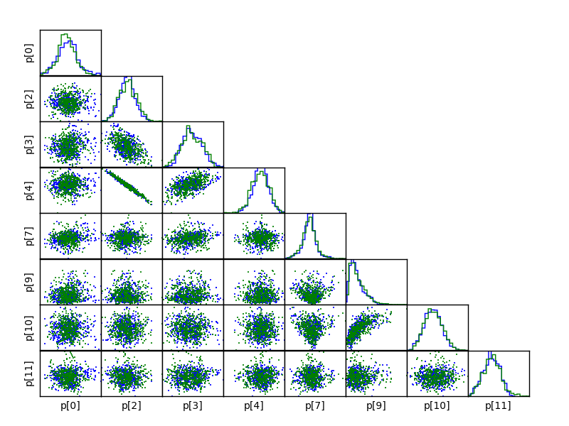
Once the chains are computed, we can extract marginalised posteriors for our parameters and make correlation plots as follows:

gp.p,gp.ep = Infer.AnalyseChains(10000,n_chains=2)

pylab.figure()
gp.plot() #plot the gp

pylab.figure()
# make correlation plots of all variable parameters
Infer.PlotCorrelations(10000,n_chains=2,p=np.where(np.array(gp.ep) > 0)[0])

which prints out a summary of the MCMC chains, and makes a plot of the correlations:

MCMC Marginalised distributions:
 par = mean gauss_err [med +err -err]: GR
 p[0] = -0.0000473 +- 0.0000949 [-0.0000499 +0.0000862 -0.0000832]: GR = 1.0023
 p[1] = 2.5000000 +- 0.0000000 [2.5000000 +0.0000000 -0.0000000]: GR = -1.0000
 p[2] = 11.0831646 +- 0.1990225 [11.0853944 +0.1956429 -0.2015135]: GR = 1.0010
 p[3] = 0.0998971 +- 0.0009834 [0.0998172 +0.0010594 -0.0008764]: GR = 1.0010
 p[4] = 0.5957373 +- 0.0196280 [0.5962324 +0.0188783 -0.0199335]: GR = 1.0005
 p[5] = 0.2000000 +- 0.0000000 [0.2000000 +0.0000000 -0.0000000]: GR = -1.0000
 p[6] = 0.3000000 +- 0.0000000 [0.3000000 +0.0000000 -0.0000000]: GR = -1.0000
 p[7] = 0.9999438 +- 0.0002570 [0.9999483 +0.0002032 -0.0002256]: GR = 1.0000
 p[8] = 0.0000000 +- 0.0000000 [0.0000000 +0.0000000 -0.0000000]: GR = -1.0000
 p[9] = 0.0004272 +- 0.0002181 [0.0003718 +0.0002609 -0.0001358]: GR = 1.0020
 p[10] = 0.0280761 +- 0.0069383 [0.0279881 +0.0070341 -0.0068133]: GR = 1.0007
 p[11] = 0.0002982 +- 0.0000166 [0.0002980 +0.0000158 -0.0000165]: GR = 1.0016
Gaussian Evidence approx:
 log ML = 1334.14509614
 log E = 1284.63138514
 log E (BIC) = 1334.14509614 - 8/2.*np.log(N)
 log E (AIC) = 1326.14509614 (D = 8, no n corr used!)